The Sliced Wasserstein Distance
This page is generated from the notebook
Sliced Wasserstein Distance.ipynbin the companion repository examples-ot, where every figure below can be reproduced and modified.
Sliced Wasserstein Distance
In this notebook, we give some more context about Figure 3 of our paper Recent Advances in Optimal Transport for Machine Learning.
References
[R1] Santambrogio, Filippo. Optimal transport for applied mathematicians. Vol. 87. Cham: Springer International Publishing, 2015.
[R2] Deshpande, I., Hu, Y. T., Sun, R., Pyrros, A., Siddiqui, N., Koyejo, S., … & Schwing, A. G. (2019). Max-sliced wasserstein distance and its use for gans. In Proceedings of the IEEE/CVF conference on computer vision and pattern recognition (pp. 10648-10656).
import ot
import numpy as np
import seaborn as sns
import matplotlib.pyplot as plt

from tqdm.auto import tqdm
from src.plot_utils import set_plot_params

set_plot_params()
np.random.seed(0)
/usr/local/lib/python3.12/dist-packages/tqdm/auto.py:21: TqdmWarning: IProgress not found. Please update jupyter and ipywidgets. See https://ipywidgets.readthedocs.io/en/stable/user_install.html
  from .autonotebook import tqdm as notebook_tqdm
Introduction
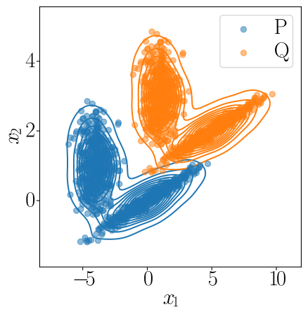
We start by creating a reference probability measure on $\mathbb{R}^{2}$, composed by two Gaussian components,
\[P = \dfrac{P_{1} + P_{2}}{2}\]and,
\(P_{1} = \mathcal{N}(\mu, \Sigma)\quad\mu = \begin{bmatrix}0 & 0\end{bmatrix}\quad\Sigma=CC^{T}\) \(P_{2} = \mathcal{N}(\mu, \Sigma)\quad\mu = \begin{bmatrix}-4 & 1\end{bmatrix}\quad\Sigma=\begin{bmatrix}0.49 & 0.00\\ 0.00 & 0.49\end{bmatrix}\)
We then generate $Q$ by pushing the samples from $P$ with $T(x) = x + b$, where $b = \begin{bmatrix} 5, 2 \end{bmatrix}$. Note that since $Q = T_{\sharp}P$, the Wasserstein distance is available in closed form. Using the Kantorovich formulation, one can show that the OT plan,
\[\gamma(x, y) = P(x)\delta(y - (x + b))\]is optimal. In this case,
\[W_{2}(P, Q)^{2} = \underset{\gamma \in \Gamma(P, Q)}{\text{inf}}\int_{\mathcal{X}}\int_{\mathcal{X}}\lVert x - y \rVert_{2}^{2}d\gamma(x, y) = \int_{\mathcal{X}}\lVert x - (x + b) \rVert_{2}^{2}dP(x) = \lVert b \rVert_{2}^{2}\]n_samples = 500
C = np.array([[0.0, -0.1], [1.7, 0.4]])
component_1 = np.dot(np.random.randn(n_samples, 2), C) # general
component_2 = 0.7 * np.random.randn(n_samples, 2) + np.array([-4, 1]) # spherical
## Reference measure
X = np.concatenate([component_1, component_2])
## Translation vector
const = np.array([5., 2.])
## Push-forward
Y = X + const
fig, ax = plt.subplots(1, 1, figsize=(5, 5))

plt.scatter(X[:, 0], X[:, 1], c="tab:blue", alpha=0.5, label="P", zorder=5)
sns.kdeplot(x=X[:, 0], y=X[:, 1], ax=ax, color="tab:blue", zorder=1)

plt.scatter(Y[:, 0], Y[:, 1], c="tab:orange", alpha=0.5, label="Q", zorder=5)
sns.kdeplot(x=Y[:, 0], y=Y[:, 1], ax=ax, color="tab:orange", zorder=1)
plt.xlabel("$x_{1}$")
plt.ylabel("$x_{2}$")
plt.legend()
<matplotlib.legend.Legend at 0x75d667342ed0>
The Sliced Wasserstein Distance
Now, we illustrate the computation of the Sliced Wasserstein distance. As a reminder,
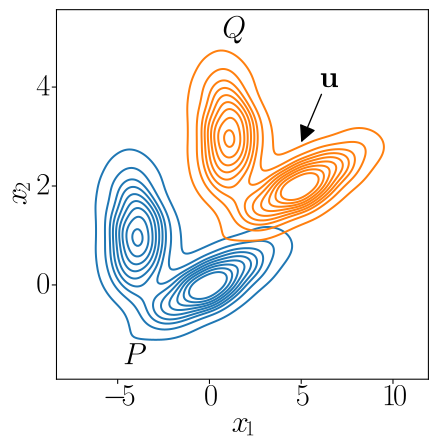
\[\text{SW}_{p}(P,Q)^{p} = \int_{\mathbb{S}^{d-1}}W_{p}(\pi_{u,\sharp}\hat{P}, \pi_{u,\sharp}\hat{Q})^{p}du\]where $u \in \mathbb{S}^{d-1} = {\mathbf{u} \in \mathbb{R}^{d}: \lVert \mathbf{u} \rVert_{2}^{2} = 1}$ and $\pi_{u}(x) = \langle u, x \rangle$. We first illustrate how this projection affects the Wasserstein distance measurement.
Note that we can randomly sample from the unit sphere by $u \sim \mathcal{N}(0, I_{2})$, then normalizing $\tilde{u} = \dfrac{u}{\lVert u \rVert_{2}}$,
p = np.random.randn(2)
p = p / np.linalg.norm(p)
This gives us a direction for which we can project the measures onto,
prop = dict(arrowstyle="-|>,head_width=0.3,head_length=0.6",
            shrinkA=0, shrinkB=0, color='k')
x_0 = np.array([6, 4])

fig, ax = plt.subplots(1, 1, figsize=(5, 5))
sns.kdeplot(x=X[:, 0], y=X[:, 1], ax=ax, zorder=5, label=r'$P$', color='tab:blue')
sns.kdeplot(x=Y[:, 0], y=Y[:, 1], ax=ax, zorder=5, label=r'$Q$', color='tab:orange')
ax.set_xlabel(r'$x_{1}$')
ax.set_ylabel(r'$x_{2}$')
ax.text(x=-4.7, y=-1.6, s=r"$P$")
ax.text(x=0.7, y=5, s=r"$Q$")
ax.annotate("$\mathbf{u}$", xy=x_0 + 1.5 * p, xytext=x_0, arrowprops=prop)
<>:12: SyntaxWarning: invalid escape sequence '\m'
<>:12: SyntaxWarning: invalid escape sequence '\m'
/tmp/ipykernel_12785/2669553973.py:12: SyntaxWarning: invalid escape sequence '\m'
  ax.annotate("$\mathbf{u}$", xy=x_0 + 1.5 * p, xytext=x_0, arrowprops=prop)


Text(6, 4, '$\\mathbf{u}$')
we now compute the Wasserstein distance in 1-D. Here, we take a little detour to explain how we can compute the 1-D version of the Wasserstein distance. For general reference, we point readers to [R1, Chapter 2] for a more complete mathematical exposition of OT in 1-D. We begin by projecting the data into $\mathbb{R}^{1}$,
Xp = np.dot(X, p)  # shape (n,)
Yp = np.dot(Y, p)  # shape (n,)
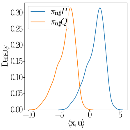
Since the data now lives in $\mathbb{R}$, we can easily estimate the densities of $\pi_{u,\sharp}P$ and $\pi_{u,\sharp}Q$,
fig, ax = plt.subplots(1, 1, figsize=(5, 5))
sns.kdeplot(Xp, ax=ax, label=r'$\pi_{\mathbf{u},\sharp}P$', c='tab:blue')
sns.kdeplot(Yp, ax=ax, label=r'$\pi_{\mathbf{u},\sharp}Q$', c='tab:orange')
ax.set_xlabel(r'$\langle \mathbf{x}, \mathbf{u} \rangle$')
ax.legend()
plt.tight_layout()
In 1-D, one can show that the following transport map,
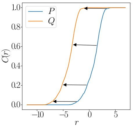
\[T_{mon}(x) = F_{Q}^{[-1]}(F_{P}(x))\]where $F_{Q}^{-1}(x) = \text{inf}{t \in \mathbb{R}: F_{Q}(t) \geq x}$ is the pseudo-inverse of the CDF $F_{Q}$ of $Q$.
In the next block of code, we compute the histgrams (which approximate the densities of $\pi_{u,\sharp}P$ and $\pi_{u,\sharp}Q$) and the respective CDFs,
bins = np.linspace(-12, 7, 100)
bin_centers = 0.5 * (bins[:-1] + bins[1:])

## Compute the densities using histograms
hX, _ = np.histogram(Xp, bins=bins, density=False)
hX = hX / hX.sum()

hY, _ = np.histogram(Yp, bins=bins, density=False)
hY = hY / hY.sum()

## Cumulative sums
cX = np.cumsum(hX)
cY = np.cumsum(hY)
Note that, since we’re on the empirical case, we can compute the infimum as a min. We only need to compute it over indices (hence we can use argsorted) to get the point that $x$ gets sent to. We illustrate the transport over the CDFs below,
fig, ax = plt.subplots(1, 1, figsize=(5, 5))

ax.plot(bin_centers, cX, c='tab:blue', label='$P$')
ax.plot(bin_centers, cY, c='tab:orange', label='$Q$')

for i in [50, 60, 70, 80, 85]:
    j = np.searchsorted(cY, cX[i])  # Finds the inf for cY[j] >= cX[i]
    if j < len(bin_centers):
        ax.annotate(
            '',
            xy=(bin_centers[j], cY[j]),
            xycoords='data',
            xytext=(bin_centers[i], cX[i]),
            textcoords='data',
            arrowprops=dict(arrowstyle= '-|>', color='k')
        )
ax.set_ylabel('$C(r)$')
ax.set_xlabel('$r$')
ax.legend()
<matplotlib.legend.Legend at 0x75d6628bccb0>
Now, note that each direction $u$ yields a different measure $P_{u} = \pi_{u,\sharp}P$, which, in turn, leads to a different value for $W_{2}(P_{u}, Q_{u})$ indexed by $u$. We can then visualize how the Wasserstein distance behaves along $\mathbb{S}^{d-1}$. In our case, since $d = 2$, we have the circle.
We start by building a matrix $U \in \mathbb{R}^{n \times d}$, where each $u_{i}$ (i.e., U[i, :]) corresponds to a vector on $\mathbb{S}^{d-1}$
U = np.random.randn(2000, 2)
U = U / np.linalg.norm(U, axis=1)[:, None]
a = np.ones(len(X)) / len(X)
b = np.ones(len(Y)) / len(Y)

w_vals = []
for u_l in U:
    Xu, Yu = np.einsum('ni,i->n', X, u_l).reshape(-1, 1), np.einsum('ni,i->n', Y, u_l).reshape(-1, 1)
    w_vals.append(ot.lp.wasserstein_1d(Xu, Yu, a, b, p=2) ** (1 / 2))
fig = plt.figure(figsize=(6, 5))
sca = plt.scatter(U[:, 0], U[:, 1], c=np.stack(w_vals).squeeze(), cmap='magma')
cbar = fig.colorbar(sca)
plt.text(0, 0, r'$S^{1}$', fontdict={'fontsize': 22}, ha='center', va='center')
plt.axis('off')
cbar.set_label(r'$W_{2}(\pi_{\mathbf{u},\sharp}P),\pi_{\mathbf{u},\sharp}Q$')
plt.tight_layout()
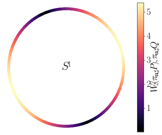
we now explore how the measure sliced-Wasserstein distance converges to the actual Wasserstein distance, depending on the number of projections we choose. Note that, if we draw $u \in \mathbb{S}^{d-1}$ at random, then $W_{2}(P_{u}, Q_{u})$ is a random variable, with a mean and standard deviation. For reference, we also compare the vanilla sliced version with the max-sliced Wasserstein distance [R2],
\[\text{max-SW}_{p}^{p}(P, Q) = \underset{\mathbf{u} \in \mathbb{S}^{d-1}}{max}W_{p}^{p}(\pi_{\mathbf{u,\sharp}}P, \pi_{\mathbf{u,\sharp}}Q)\]sw_means = []
sw_stds = []
max_sw_means = []
max_sw_stds = []
n = np.logspace(0, 3, num=20, base=10, dtype=int)
for n_proj in tqdm(n):
sw_estimates = []
max_sw_estimates = []
for _ in range(5):
U = np.random.randn(n_proj, 2)
U = U / np.linalg.norm(U, axis=1)[:, None]
w_vals = []
for u_l in U:
Xu, Yu = np.einsum('ni,i->n', X, u_l).reshape(-1, 1), np.einsum('ni,i->n', Y, u_l).reshape(-1, 1)
w_vals.append(ot.lp.wasserstein_1d(Xu, Yu, a, b, p=2) ** (1 / 2))
sw_estimates.append(np.stack(w_vals).squeeze().mean())
max_sw_estimates.append(np.stack(w_vals).squeeze().max())
sw_means.append(np.mean(sw_estimates))
sw_stds.append(np.std(sw_estimates))
max_sw_means.append(np.mean(max_sw_estimates))
max_sw_stds.append(np.std(max_sw_estimates))
sw_means = np.array(sw_means)
sw_stds = np.array(sw_stds)
max_sw_means = np.array(max_sw_means)
max_sw_stds = np.array(max_sw_stds)
plt.figure(figsize=(5, 5))
plt.plot(n, sw_means, label=r'$SW_{2}$', c='tab:blue')
plt.plot(n, max_sw_means, label=r'$max-SW_{2}$', c='tab:orange')
plt.plot(n, len(n) * [np.linalg.norm(const),], 'k--', label="$W_{2}$")
plt.fill_between(n, sw_means - 2 * sw_stds, sw_means + 2 * sw_stds, alpha=0.1, facecolor='tab:blue')
plt.fill_between(n, max_sw_means - 2 * max_sw_stds, max_sw_means + 2 * max_sw_stds, alpha=0.1, facecolor='tab:orange')
plt.ylabel('Distance')
plt.xlabel('Number of Projections')
plt.xscale('log')
plt.legend()
<matplotlib.legend.Legend at 0x75d661e2ab70>
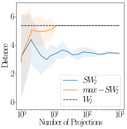
Note that, while the max-SW distance converges to the true Wasserstein distance, the sliced version is a biased estimator, i.e., it converges to a value different from $W_{2}$.